
 by
by Models that impact people’s lives must be honest and forthcoming about their doubts. This new method brings balance to explainable AI.
This article was originally posted on Towards Data Science
At Featurespace, we have published a method for explaining model uncertainties in deep networks. Our approach makes it possible to understand the confounding patterns in the input data that a model believes do not fit with the class it predicts. This allows us to deploy honest and transparent models that give balanced and complete evidence for a decision, rather than just curating the evidence in support of its decision.
For example, in the figure below we observe three images of celebrities contained within the CelebA dataset. In all cases, the celebrities are labelled as “not smiling”, which is easily predicted using widely available deep classification models for image processing tasks, such as VGG16, ResNet50 or EfficientNet. However, models can struggle to offer confident classifications for some of these pictures. In the examples below, our proposed method highlights the various features that caused models to be uncertain (right column). We readily notice the presence of smile arcs, upper lip curvatures and buccal corridors commonly associated with smiles and grins.
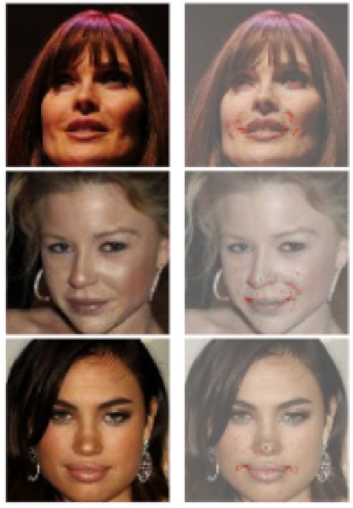
Left: images of celebrity faces in the CelebA dataset with predicted class label ‘no smile’. Right: pixels highlighted by our approach (red) that caused the model to be uncertain about that prediction. Images by author.
Uncertainty and Bayesian Deep Learning
We built our uncertainty attribution method on top of Bayesian neural networks, (BNNs). This framework thoroughly treats all of the sources of uncertainty in a prediction including the uncertainty emanating from the model choice and limitations of the training data, which emerges as uncertainty on the fitted weight parameters of every neural cell. A good overview of BNNs is available here. In summary:
- Every fitted parameter for a neuron is captured as a probability distribution that represents our lack of certainty regarding its best value, given the training data.
- Since a deep model has plenty of parameters, thus, we have a multivariate distribution over all trained parameters, referred to as the posterior distribution.
- When we classify a new data point, each plausible combination of fitted parameter values offers us a different score! Rather than a single score, the BNN offers us a distribution of possible scores, called the posterior predictive distribution.
- BNNs commonly return the mean of the posterior predictive distribution as their estimate of the output score.
These computations are often approximated and run under the hood, for example, when you add dropout layers into your neural model architecture. The important thing is, for every image, piece of text or financial transaction that we wish to classify, we may retrieve a distribution that represents what a score should be. A pair of example distributions for MNIST digits is shown below. The means of the distributions tells us how “certain” the classification is, while the variance tells us how “stable” it is to modelling uncertainties. Note that the mean score can sometimes be quite different to the score produced by the most likely set of model parameters, which is what non-Bayesian neural networks typically return. The deviation of most-likely model vs mean-model scores is particularly high in the first example.
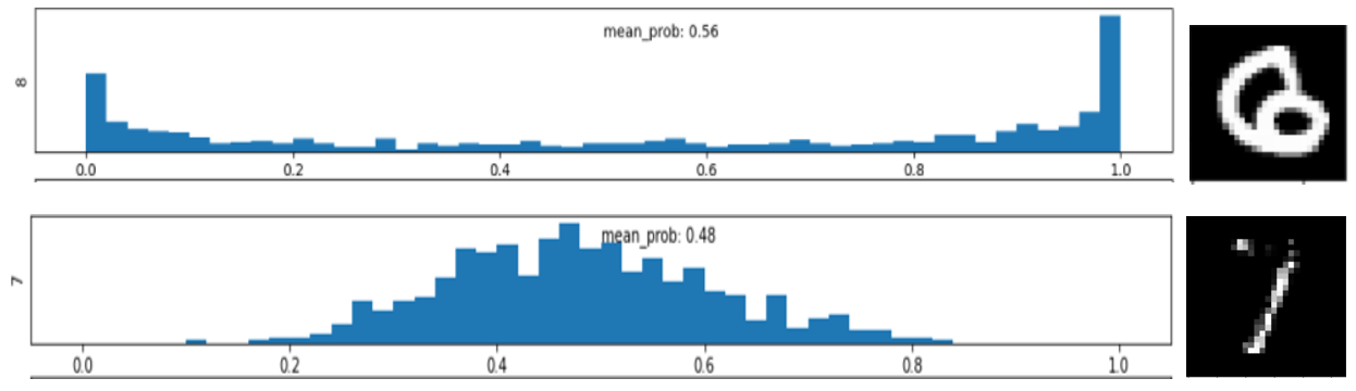
Posterior predictive distributions for the underlying class prevalence for two MNIST digits with similar BNN probabilities for the most likely class. In the top image, the distribution shown (for the class label ‘8’) supports a wide range of possible scores, in fact it is bimodal, favouring either certainty that the image has to be an ‘8’, or certainty that it cannot possibly be an ‘8’. This implies the image is representative of a sparse region in the data with few or no exemplars in the training set. In contrast, the distribution in the bottom image is peaked around 0.5 and is relatively narrow. This implies the training set contains evidence of intrinsic class mixture at this point in the feature space — it has seen similar examples that have either been labelled as (incomplete) ‘7’s or as ‘1’s with a stray blobs of peripheral ink. Images by author.
Explaining Model Uncertainty
To explain the uncertainty in a prediction, our approach builds on the framework of integrated gradients (Sundararajan et al. 2017), one of the most widespread explanation techniques for neural networks. Integrated gradients works by integrating the gradient of the model’s output propensity score pc(x) for class c. It performs this integration along a path in the feature space between a fiducial starting point and the point being explained. For uncertainty explanation, instead of integrating the gradient of the model score, we integrate the gradient of the predictive entropy
H(x)= -Σc pc(x) . log pc(x)
This measure encapsulates the total predictive uncertainty of the model, including components emanating from both the location and width of the posterior predictive distribution.
We tested integrated entropy gradients on public image benchmarks, including MNIST and the CelebA faces datasets. Unfortunately, the entropy explanations produced by vanilla integrated gradients turned out to be poor, confusing and of an adversarial kind. This is understandable, integrated gradients requires a fiducial feature vector as the origin of the path integral, and the vanilla algorithm uses a blank image as its fiducial. This has reasonable motivations for explaining why a score is high because the blank image is likely to have a roughly equal model score for all classes; however, the uncertainty surrounding a black image is commonly very high.
To overcome this and other problems (details of these are in the paper), our approach combines two recent ideas to produce clean and informative entropy attributions — Both of which make use of a latent space learnt representation, using a variational autoencoder.
- Synthesised counterfactual explanations (Antoran et al. 2021). For our path integral’s source image, we want an image that has the same predicted class as our test image, but with zero predictive entropy. A synthesised counterfactual explanation image provides such a source image, while having the attractive property that the source image bears very close resemblance to the test image — that is, the delta is restricted to those concepts that drive up the uncertainty.
- In-distribution path integrals (Jha et al. 2020) One problem with integrated gradients is that the path between fiducial source and test vectors may stray off the data manifold — exploring a track through impossible images. We want the path integral between fiducial and test points to be within the data manifold, ie: every feature vector on the path between the two images is representative of something that might reasonably occur in the data.
In combination, these ideas produce clean and relevant uncertainty explanations, even for difficult machine learning problems such as reading human expressions. We demonstrate this by explaining the most uncertain images in tasks like smile detection, arched eyebrow detection, and bags-under-eyes detection, in the CelebA dataset.
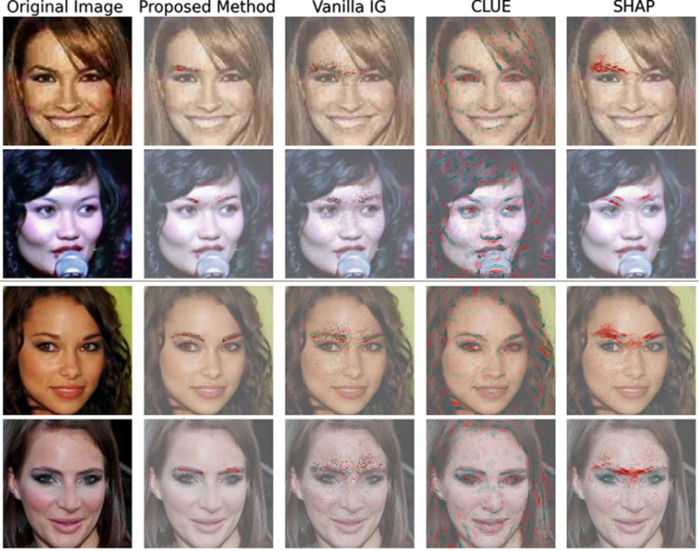
Uncertainty explanations from our method compared to existing methods for the prediction ‘arched eyebrows’ (top two rows) and ‘no arched eyebrows’ (bottom two rows). Images by author.
Conclusion
The emerging field of explainable AI typically focusses on assembling evidence that supports the decision that has been made, like a lawyer presenting a case in court. However, most AI models operate more like expert witnesses than lawyers persuading a judge. This establishes a clear need for more balanced explanation approaches that offer nuanced explanations articulating fuzziness, uncertainty and doubt. What our approach does is to complement traditional score attribution approaches with a rich but concise explanation for why a data point’s classification is not certain. As machine learning is used more widely to inform legal, financial, or medical decisions that have a large impact on lives, an honest and open appraisal of the weight of evidence behind automated predictions will be vital for maintaining ethical standards.
Featurespace’s Piotr Skalski will be at this year’s uai2022 event (Aug 1-5), presenting his research paper ‘Attribution of Predictive Uncertainties in Classification Models’. Download the full paper here.
Share